---
title: "Does spending more money win more votes? Moldova's 2025 elections"
description: "This blog post asks a simple question: did the parties and candidates that spent more money in Moldova's 2025 parliamentary elections also get more votes? It shows how much spending goes with a given vote share, and what the chances of reaching the 5% threshold were at different spending levels. It is the third post based on my analysis in the Moldovan Analytical Digest."
author:
  - name: Sergiu Lipcean
    url: https://sergiulipcean.github.io/
    orcid: 0000-0002-8944-6505
date: "2026-05-23"
categories: [campaign finance, campaign spending, electoral returns, elections, Moldova] # self-defined categories
draft: false # setting this to `true` will prevent the post from appearing on the listing page!
link-citations: true
csl: apa.csl
linkcolor: "#0F4D92"
urlcolor: "#0F4D92"
bibliography: references.bib
---

```{=html}
<style type = text/css>
  body{line-height: 1.5em;
  font-size: 14pt;
  font-family: Trebuchet MS;
  text-align: justify;}
</style>
```

```{r setup, include=FALSE}
knitr::opts_chunk$set(echo = FALSE, warning = FALSE, message = FALSE, fig.width = 10, fig.height = 10, dev = "ragg_png")
```

```{r}
# Download R packages
library(tidyverse)
library(openxlsx)
library(brms)
library(tidybayes)
library(marginaleffects)
library(betareg)
library(ggrepel)
library(scales)
library(extrafont)

# Make the Windows fonts available to the plots (Trebuchet MS, as in the text)
loadfonts(device = "win", quiet = TRUE)
```

```{r}
# Spending and vote shares: one row per electoral contestant (21 contestants)
# Spending is converted from lei to thousand euro (MDL 19.5 per euro)
# "Total" includes the value of volunteer work, "monetary" leaves it out
d <- read.xlsx("spending_returns.xlsx") %>%
  mutate(percentage_prop = percentage / 100,
         total_k    = round(total_expenses / 19.5 / 1000, 2),
         monetary_k = round((total_expenses - volunteer_value) / 19.5 / 1000, 2),
         cleared    = percentage >= 5)

# One data set per spending measure, with the same variable names, so that the models use the same formulas
# log_spend = log of spending in thousand euro; x = log_spend centred and divided by its standard deviation
data_models <- list(
  "Total spending"    = d %>% mutate(log_spend = log(total_k)),
  "Monetary spending" = d %>% mutate(log_spend = log(monetary_k))) %>%
  map(~ mutate(.x, x = (log_spend - mean(log_spend)) / sd(log_spend)))

# Mean and standard deviation of log spending (to move between the two scales) and the highest spending observed
scale_tbl <- data_models %>%
  map(~ summarise(.x, mu = mean(log_spend), sdv = sd(log_spend), max_spend = max(exp(log_spend)))) %>%
  list_rbind(names_to = "measure")
```

```{r}
#| cache: false

# Bayesian beta regression with a quadratic term in standardised log spending
# Weakly informative priors: Normal(0, 1) on standardised spending lets the data decide
priors <- c(prior(normal(-4, 1.5), class = Intercept),
            prior(normal(0, 1), class = b),
            prior(gamma(2, 0.1), class = phi))

# The fitted models are saved in the folder "fits", so they are only estimated the first time
fit_total <- brm(
  percentage_prop ~ x + I(x^2),
  data = data_models[["Total spending"]], family = Beta(), prior = priors,
  chains = 4, iter = 5000, warmup = 2500, seed = 123,
  control = list(adapt_delta = 0.99, max_treedepth = 15),
  backend = "cmdstanr", refresh = 0, silent = 2, file = "fits/bayes_total")

fit_monetary <- brm(
  percentage_prop ~ x + I(x^2),
  data = data_models[["Monetary spending"]], family = Beta(), prior = priors,
  chains = 4, iter = 5000, warmup = 2500, seed = 123,
  control = list(adapt_delta = 0.99, max_treedepth = 15),
  backend = "cmdstanr", refresh = 0, silent = 2, file = "fits/bayes_monetary")

bayes_models <- list("Total spending|Bayesian"    = fit_total,
                     "Monetary spending|Bayesian" = fit_monetary)

# The same model estimated the simple way (one best-fit curve), as in the digest analysis, used as a check
freq_models <- list(
  "Total spending|simple" =
    betareg(percentage_prop ~ log_spend + I(log_spend^2) | log_spend, data = data_models[["Total spending"]]),
  "Monetary spending|simple" =
    betareg(percentage_prop ~ log_spend + I(log_spend^2) | log_spend, data = data_models[["Monetary spending"]]))
```

```{r}
# Fix the random seed so that the numbers in the text are the same every time the page is rendered
set.seed(123)

# Grids of spending levels (log scale), plus a few values used in the text; predictions are restricted to the observed range
grid <- tibble(log_spend = sort(unique(c(seq(log(2), log(1500), length.out = 200),
                                         log(c(50, 100, 200, 300, 500))))))

grid_fine <- tibble(log_spend = seq(log(2), log(1500), length.out = 500))

grid_measure <- scale_tbl %>%
  cross_join(grid) %>%
  mutate(x = (log_spend - mu) / sdv, spend = exp(log_spend)) %>%
  filter(spend <= max_spend)

grid_fine_measure <- scale_tbl %>%
  cross_join(grid_fine) %>%
  mutate(x = (log_spend - mu) / sdv, spend = exp(log_spend)) %>%
  filter(spend <= max_spend)

# Expected vote share for every spending level and every one of the thousands of possible curves
epred <- bayes_models %>%
  imap(~ add_epred_draws(filter(grid_measure, measure == str_extract(.y, "^[^|]+")) %>% select(-measure),
                         .x, ndraws = 2000, dpar = "phi")) %>%
  list_rbind(names_to = "model") %>%
  separate_wider_delim(model, "|", names = c("measure", "approach")) %>%
  mutate(measure = factor(measure, levels = c("Total spending", "Monetary spending")))

# Chance of getting at least 5% of the votes at each spending level:
# for every curve, the probability that a vote share drawn from the beta distribution is at least 5%, averaged over curves
p_clear <- epred %>%
  mutate(p = 1 - pbeta(0.05, .epred * phi, (1 - .epred) * phi)) %>%
  summarise(p_clear = mean(p), .by = c(measure, spend))

# Spending level beyond which the expected vote share stays above 5% (for every curve)
crossing <- bayes_models %>%
  imap(~ add_epred_draws(filter(grid_fine_measure, measure == str_extract(.y, "^[^|]+")) %>% select(-measure),
                         .x, ndraws = 1000)) %>%
  list_rbind(names_to = "model") %>%
  separate_wider_delim(model, "|", names = c("measure", "approach")) %>%
  filter(.epred < 0.05) %>%
  mutate(measure = factor(measure, levels = c("Total spending", "Monetary spending"))) %>%
  summarise(spend_5pct = max(spend), .by = c(measure, approach, .draw))

crossing_summary <- crossing %>%
  group_by(measure, approach) %>%
  median_qi(spend_5pct) %>%
  mutate(key = paste(measure, approach, sep = "|")) %>%
  column_to_rownames("key")

# Expected vote share at selected spending levels
share_summary <- epred %>%
  filter(round(spend, 6) %in% c(100, 300, 500)) %>%
  mutate(spend = round(spend, 6)) %>%
  group_by(measure, approach, spend) %>%
  mutate(share = .epred * 100) %>%
  median_qi(share) %>%
  mutate(key = paste(measure, approach, spend, sep = "|")) %>%
  column_to_rownames("key")

# The same spending level from the simple model
freq_crossing <- freq_models %>%
  imap(~ filter(grid_fine_measure, measure == str_extract(.y, "^[^|]+")) %>%
         mutate(estimate = predict(.x, newdata = pick(everything()), type = "response")) %>%
         select(-measure)) %>%
  list_rbind(names_to = "model") %>%
  separate_wider_delim(model, "|", names = c("measure", "approach")) %>%
  filter(estimate < 0.05) %>%
  summarise(spend_5pct = max(spend), .by = c(measure, approach)) %>%
  mutate(key = paste(measure, approach, sep = "|")) %>%
  column_to_rownames("key")

# Effect of doubling spending, at different starting levels (difference in expected vote share, percentage points)
# On the standardised scale a doubling is a change of log(2) divided by the standard deviation of log spending
effects <- bayes_models %>%
  imap(~ comparisons(.x,
                     variables = list(x = log(2) / scale_tbl$sdv[scale_tbl$measure == str_extract(.y, "^[^|]+")]),
                     newdata = datagrid(model = .x,
                                        x = (log(c(25, 50, 100, 200, 400)) - scale_tbl$mu[scale_tbl$measure == str_extract(.y, "^[^|]+")]) /
                                          scale_tbl$sdv[scale_tbl$measure == str_extract(.y, "^[^|]+")]),
                     type = "response") %>%
         posterior_draws()) %>%
  list_rbind(names_to = "model") %>%
  separate_wider_delim(model, "|", names = c("measure", "approach")) %>%
  left_join(scale_tbl, by = "measure") %>%
  mutate(measure = factor(measure, levels = c("Total spending", "Monetary spending")),
         start = round(exp(x * sdv + mu)),
         change = draw * 100)

effects_summary <- effects %>%
  group_by(measure, start) %>%
  median_qi(change) %>%
  mutate(key = paste(measure, start, sep = "|")) %>%
  column_to_rownames("key")

# Convergence checks of the models
rhat_max <- max(rhat(fit_total), rhat(fit_monetary))
divergences <- sum(subset(nuts_params(fit_total), Parameter == "divergent__")$Value,
                   subset(nuts_params(fit_monetary), Parameter == "divergent__")$Value)
```

This is the third post based on my analysis in the Moldovan Analytical Digest [@lipcean2026]. The [first](../2026-03-15-moldova-2025-campaign-income/index.qmd) and [second](../2026-04-18-moldova-2025-campaign-spending/index.qmd) posts examined how the parties and candidates in Moldova's 2025 parliamentary elections gathered their campaign funds and how they spent them, so here I turn to the question that naturally follows: **did the contestants with the deepest pockets also obtain the most votes?**

The short answer is yes, but mainly at the top of the spending ladder. Contestants running on a very limited budget attracted very few votes, whereas the big spenders secured far more. In addition, the more funding a contestant had already invested, the more support each additional euro appeared to bring. With only `r nrow(d)` contestants, however, it is nearly impossible to say precisely how much money one needed to invest for a given vote share.

::: {.callout-note collapse="true"}
## Acronyms of electoral contestants

```{r}
read.xlsx("acronims.xlsx") %>%
  rename(Acronym = party_acronym, `Electoral contestant` = party_name_en) %>%
  knitr::kable()
```
:::

***A preliminary glance of the data***

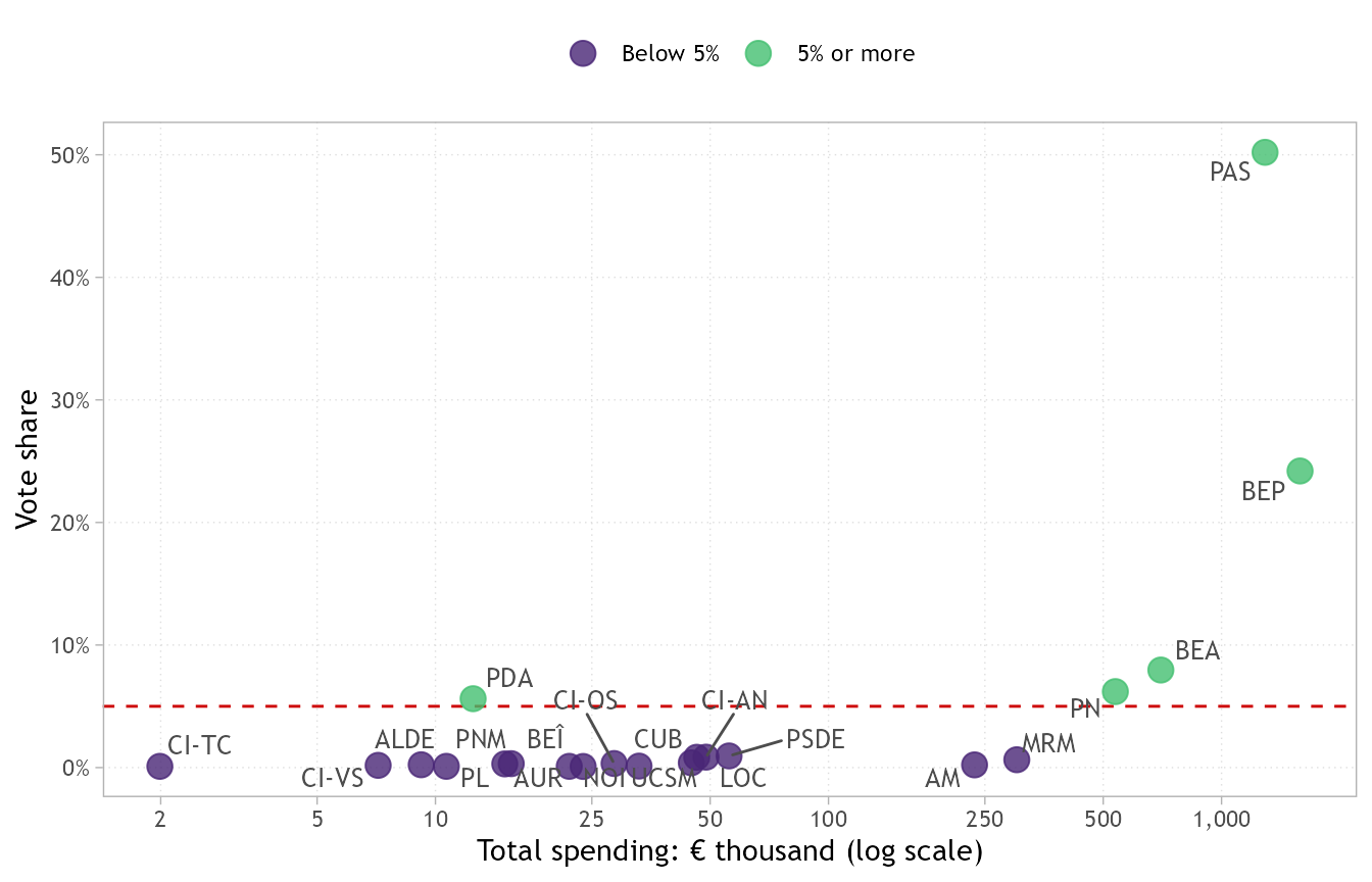
@fig-data plots, for each contestant, how much it spent against the share of the votes it obtained. I measure spending in two ways: *monetary spending*, which counts only the cash actually spent and *total spending*, which also includes the value of activities carried out by volunteers. @fig-data presents the information on total spending. Since spending varies enormously, from less than €2,000 to more than €1.5 million, the x-axis uses a logarithmic scale, thus helping to show small and large spenders against their vote shares in the same picture. Each dot is a contestant, and the dashed red line marks the 5% threshold required to enter parliament, so the green dots above the line are the contestants that cleared the electoral threshold.

Overall, contestants that spent more gained more votes, while the four biggest spenders all surpassed 5%. Yet the picture is not as clear as one may expect. For instance, the Democracy at Home Party (PDA) cleared the threshold with only about €12,500, while the Moldovans Alliance (AM) and Respect Moldova Movement (MRM) poured about €235 thousand and €300 thousand into their campaign chests respectively, but collected less than 1% of the votes.

```{r}
#| label: fig-data
#| fig-cap: "Campaign spending and vote share of electoral contestants in Moldova's 2025 parliamentary elections. Spending includes the value of volunteer work and is shown on a logarithmic scale. The dashed line is the 5% threshold."
#| fig-alt: "A scatter plot where each point is an electoral contestant, placed by total spending in thousand euro (logarithmic axis) and vote share. Contestants that got 5 percent or more are in a different colour; spending and vote share are positively related."
#| fig-height: 4.5
#| fig-width: 7

d %>%
  ggplot(aes(x = total_k, y = percentage_prop, colour = cleared)) +
  geom_hline(yintercept = 0.05, linetype = 2, colour = "red3") +
  geom_point(size = 4, alpha = 0.8) +
  geom_text_repel(aes(label = party_acronym), colour = "grey30", size = 3.5, family = "Trebuchet MS") +
  scale_x_log10(breaks = c(2, 5, 10, 25, 50, 100, 250, 500, 1000), labels = comma) +
  scale_y_continuous(labels = percent) +
  scale_colour_viridis_d(name = "", labels = c("Below 5%", "5% or more"), begin = 0.1, end = 0.7) +
  labs(x = "Total spending: € thousand (log scale)", y = "Vote share") +
  theme_light(base_family = "Trebuchet MS") +
  theme(panel.grid.minor = element_blank(),
        panel.grid.major = element_line(linetype = 3),
        legend.position = "top")
```

***How many votes does spending go with?***

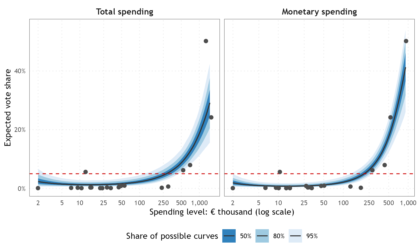
To uncover the overall pattern behind the dots in @fig-data, I fitted a **Bayesian beta regression** to the data, which is a model suited to outcomes that are proportions, like the vote share in our case. A key difference from a standard **Beta regression** is that instead of estimating a single best-fit line, the Bayesian model generates thousands of plausible lines consistent with the data. @fig-predictions shows these lines for total and monetary spending. The solid line is the median of those plausible lines produced by the model, while the shaded bands show the ranges containing 50%, 80%, and 95% of them.

A contestant spending €100 thousand is expected to obtain about `r round(share_summary["Total spending|Bayesian|100", "share"], 1)`% of the votes (most likely between `r round(share_summary["Total spending|Bayesian|100", ".lower"], 1)`% and `r round(share_summary["Total spending|Bayesian|100", ".upper"], 1)`%), whereas with €500 thousand the expected share increases to about `r round(share_summary["Total spending|Bayesian|500", "share"], 1)`% (between `r round(share_summary["Total spending|Bayesian|500", ".lower"], 1)`% and `r round(share_summary["Total spending|Bayesian|500", ".upper"], 1)`%). The model is more uncertain at high spending levels, simply because fewer contestants spent large amounts relative to more contestants that spent much less. If one takes only monetary spending, €500 thousand corresponds to roughly `r round(share_summary["Monetary spending|Bayesian|500", "share"], 1)`% of the votes.

```{r}
#| label: fig-predictions
#| fig-cap: "Expected vote share by spending level in Moldova's 2025 parliamentary elections. The line is the middle estimate, the bands show where 50%, 80% and 95% of the possible curves fall. Points are the contestants; the dashed line is the 5% threshold. Curves stop at the highest spending observed for each measure."
#| fig-alt: "Two panels, one for total spending and one for monetary spending, each with a rising curve of expected vote share against spending in thousand euro on a logarithmic axis, with blue bands that widen at high spending, and the contestants as points."
#| fig-height: 4.5
#| fig-width: 7.5

points <- bind_rows("Total spending"    = d %>% transmute(party_acronym, spend = total_k, percentage_prop),
                    "Monetary spending" = d %>% transmute(party_acronym, spend = monetary_k, percentage_prop),
                    .id = "measure") %>%
  mutate(measure = factor(measure, levels = c("Total spending", "Monetary spending")))

epred %>%
  ggplot(aes(x = spend, y = .epred)) +
  stat_lineribbon(.width = c(0.5, 0.8, 0.95), colour = "grey20", linewidth = 0.6) +
  geom_hline(yintercept = 0.05, linetype = 2, colour = "red3") +
  geom_point(data = points, aes(y = percentage_prop), size = 2, colour = "grey30") +
  scale_fill_brewer(palette = "Blues", name = "Share of possible curves",
                    labels = c("95%", "80%", "50%"),
                    guide = guide_legend(reverse = TRUE)) +
  scale_x_log10(breaks = c(2, 5, 10, 25, 50, 100, 250, 500, 1000), labels = comma) +
  scale_y_continuous(labels = percent, limits = c(0, 0.6), oob = scales::oob_keep) +
  facet_wrap(~ measure, scales = "free_x") +
  labs(x = "Spending level: € thousand (log scale)", y = "Expected vote share") +
  coord_cartesian(ylim = c(0, 0.55)) +
  theme_minimal(base_family = "Trebuchet MS") +
  theme(legend.position = "bottom",
        strip.text = element_text(size = 11, face = "bold"),
        panel.border = element_rect(colour = "grey50", fill = NA),
        panel.grid.minor = element_blank(),
        panel.grid.major = element_line(linetype = 3))
```

***Does each extra euro buy more votes?***

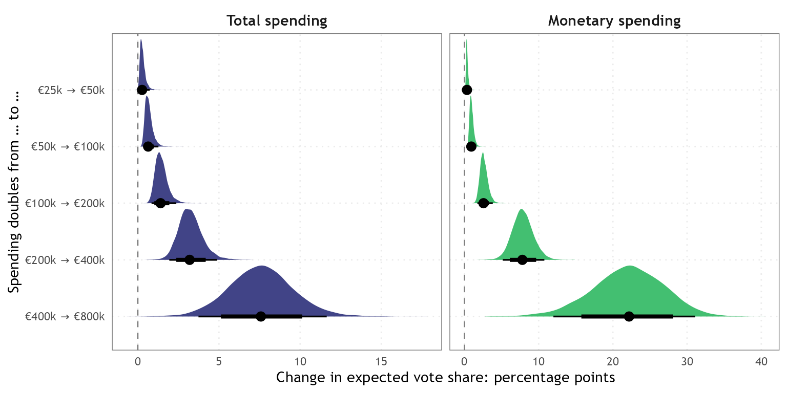
The steepening of the curve implies that the more a contestant has already spent, the more votes an additional euro appears to buy. To illustrate, consider a contestant that doubles its spending and ask how much its vote share would increase. @fig-effects answers this for five starting levels, from €25,000 to €400,000. Each marker depicts the range of plausible gains in percentage points: the dot is the middle estimate, the thick and thin lines contain 80% and 95% of the plausible values, and the dashed line marks no change.

A contestant starting at €25 thousand that doubles its budget to €50 thousand gains only about `r round(effects_summary["Total spending|25", "change"], 1)` percentage points in vote share, whereas one starting at €200 thousand and doubling to €400 thousand gains about `r round(effects_summary["Total spending|200", "change"], 1)` percentage points. In other words, votes are not bought at a fixed price: extra spending has little effects on electoral gains at lower spending levels but matters far more at higher ones. This somewhat sustains the idea that large budgets unlock expensive but effective campaign tools, such as TV advertising and professional campaigns, that small budgets cannot afford. Yet, as the @fig-effects shows, the model is also significantly more uncertain about the size of electoral gains at higher spending levels as illustrated by a wider range of plausible values for the well-funded contestants.

```{r}
#| label: fig-effects
#| fig-cap: "Change in expected vote share (percentage points) when spending doubles, starting from different spending levels in Moldova's 2025 parliamentary elections (dot: middle estimate; thick and thin lines: 80% and 95% plausible ranges)."
#| fig-alt: "Two panels with distributions of the change in vote share, in percentage points, when spending doubles from five starting levels between 25 and 400 thousand euro. The effect and its uncertainty both grow with the starting level."
#| fig-height: 4
#| fig-width: 8

effects %>%
  mutate(start_label = fct_reorder(paste0("€", start, "k → €", start * 2, "k"), start)) %>%
  ggplot(aes(x = change, y = fct_rev(start_label), fill = measure)) +
  geom_vline(xintercept = 0, linetype = 2, colour = "grey50") +
  stat_halfeye(.width = c(0.8, 0.95), point_interval = median_qi,
               normalize = "xy", scale = 0.9) +
  scale_fill_viridis_d(begin = 0.2, end = 0.7) +
  facet_wrap(~ measure, scales = "free_x") +
  guides(fill = "none") +
  labs(x = "Change in expected vote share: percentage points", y = "Spending doubles from … to …") +
  theme_minimal(base_family = "Trebuchet MS") +
  theme(strip.text = element_text(size = 11, face = "bold"),
        panel.border = element_rect(colour = "grey50", fill = NA),
        panel.grid.minor = element_blank(),
        panel.grid.major = element_line(linetype = 3))
```

***What were the chances of getting into parliament?***

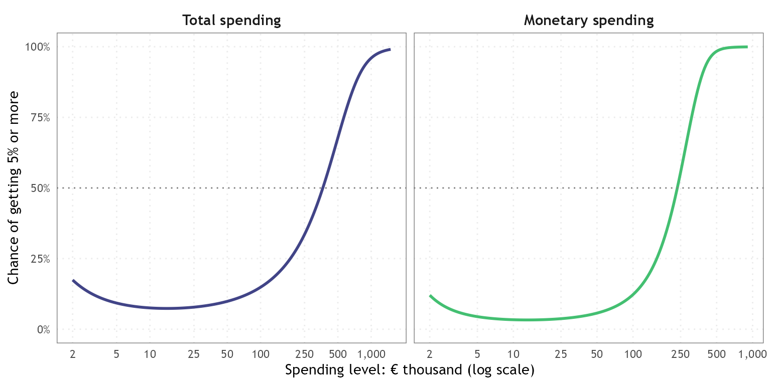
The curve in @fig-predictions is the model’s central estimate of the vote share, depending exclusively on the money spent. However, electoral success and actual votes a contestant obtains also hinges on factors the model does not know, including the quality of the contestants, public recognition, whether they are in government or in opposition or plain luck. @fig-probability takes this uncertainty into account and shows, for each spending level, the *chance* of winning at least 5% of the votes.

For instance, contestants spending €100 thousand have a chance of clearing electoral threshold of about `r percent(p_clear$p_clear[p_clear$measure == "Total spending" & round(p_clear$spend, 6) == 100], accuracy = 1)`, for those spending €300 thousand the chance jumps to `r percent(p_clear$p_clear[p_clear$measure == "Total spending" & round(p_clear$spend, 6) == 300], accuracy = 1)`, while with €500 thousand it increases to `r percent(p_clear$p_clear[p_clear$measure == "Total spending" & round(p_clear$spend, 6) == 500], accuracy = 1)`. Even contestants with the smallest budgets have a chance of passing the threshold of around `r percent(min(p_clear$p_clear[p_clear$measure == "Total spending"]), accuracy = 1)`, which fits the case of PDA - a highly unlikely case, but it happened.

```{r}
#| label: fig-probability
#| fig-cap: "Chance of getting at least 5% of the votes by spending level in Moldova's 2025 parliamentary elections. The curve is averaged over all the possible curves of the model."
#| fig-alt: "Two panels with a rising curve of the chance of reaching 5 percent of the votes against spending in thousand euro on a logarithmic axis, one for total and one for monetary spending, starting around 10 percent and approaching 100 percent for high spending."
#| fig-height: 4
#| fig-width: 8

p_clear %>%
  ggplot(aes(x = spend, y = p_clear, colour = measure)) +
  geom_line(linewidth = 1) +
  geom_hline(yintercept = 0.5, linetype = 3, colour = "grey50") +
  scale_colour_viridis_d(begin = 0.2, end = 0.7) +
  scale_x_log10(breaks = c(2, 5, 10, 25, 50, 100, 250, 500, 1000), labels = comma) +
  scale_y_continuous(labels = percent, limits = c(0, 1)) +
  facet_wrap(~ measure, scales = "free_x") +
  labs(x = "Spending level: € thousand (log scale)", y = "Chance of getting 5% or more") +
  theme_minimal(base_family = "Trebuchet MS") +
  theme(legend.position = "none",
        strip.text = element_text(size = 11, face = "bold"),
        panel.border = element_rect(colour = "grey50", fill = NA),
        panel.grid.minor = element_blank(),
        panel.grid.major = element_line(linetype = 3))
```

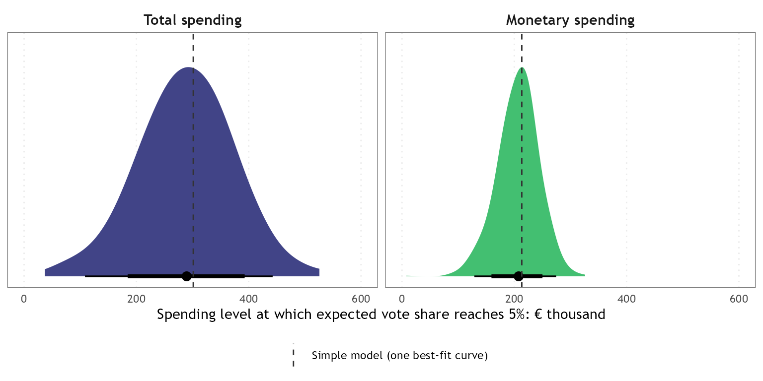
So how much does a contestant need to spend before it can *expect* to reach 5%? Each of the thousands of possible curves crosses the 5% line at a different spending level, and @fig-crossing shows how these spending levels are spread out. The black dot is the middle estimate, the thick and thin lines contain 80% and 95% of the possible values, while the dashed vertical line shows the estimate of a simpler beta model, which generates very close estimates, at about €`r round(freq_crossing["Total spending|simple", "spend_5pct"])` thousand for the total spending model and about €`r round(freq_crossing["Monetary spending|simple", "spend_5pct"])` thousand for the monetary spending one. Hence, the Bayesian model gives slightly lower estimates of the spending needed to reach 5% than the simpler beta model, although the difference is small compared with the range of plausible values.

For the **total spending** (left-hand panel), the middle estimate is about €`r round(crossing_summary["Total spending|Bayesian", "spend_5pct"])` thousand, but it could plausibly lie anywhere between €`r round(crossing_summary["Total spending|Bayesian", ".lower"])` thousand and €`r round(crossing_summary["Total spending|Bayesian", ".upper"])` thousand. For the monetary **spending model** (right-hand panel), the middle estimate is about €`r round(crossing_summary["Monetary spending|Bayesian", "spend_5pct"])` thousand (between €`r round(crossing_summary["Monetary spending|Bayesian", ".lower"])` and €`r round(crossing_summary["Monetary spending|Bayesian", ".upper"])` thousand). Given the wide range of plausible spending values, with `r nrow(d)` contestants it is hard to say accurately how much money a competitor needed to spend to clear the electoral threshold. Yet we know from the data that it required a rather hefty campaign budget.

```{r}
#| label: fig-crossing
#| fig-cap: "Spending level beyond which the expected vote share stays above 5%, in Moldova's 2025 parliamentary elections. The distribution is from the Bayesian model (dot: middle estimate; thick and thin lines: 80% and 95% plausible ranges). The dashed line represents the estimate from a simple beta regression model."
#| fig-alt: "Two panels showing the distribution of the spending level in thousand euro at which the expected vote share reaches 5 percent, for total and monetary spending. The distributions are wide, with the simple model estimate as a vertical line inside them."
#| fig-height: 4
#| fig-width: 8

freq_lines <- freq_crossing %>%
  rownames_to_column("key") %>%
  mutate(measure = factor(measure, levels = c("Total spending", "Monetary spending")))

crossing %>%
  ggplot(aes(x = spend_5pct, fill = measure)) +
  stat_halfeye(.width = c(0.8, 0.95), point_interval = median_qi,
               normalize = "xy", scale = 0.9, adjust = 1.5) +
  geom_vline(data = freq_lines, aes(xintercept = spend_5pct, linetype = approach),
             colour = "grey20") +
  scale_fill_viridis_d(begin = 0.2, end = 0.7) +
  scale_linetype_manual(values = c("simple" = 2),
                        labels = c("simple" = "Simple model (one best-fit curve)"),
                        name = "") +
  scale_x_continuous(labels = comma, limits = c(0, 600), oob = scales::oob_keep) +
  coord_cartesian(xlim = c(0, 600)) +
  scale_y_continuous(breaks = NULL) +
  facet_wrap(~ measure, scales = "free_x") +
  guides(fill = "none") +
  labs(x = "Spending level at which expected vote share reaches 5%: € thousand", y = NULL) +
  theme_minimal(base_family = "Trebuchet MS") +
  theme(legend.position = "bottom",
        strip.text = element_text(size = 11, face = "bold"),
        panel.border = element_rect(colour = "grey50", fill = NA),
        panel.grid.minor = element_blank(),
        panel.grid.major = element_line(linetype = 3))
```

***What this does not tell us***

These numbers show how spending and votes moved together in this parliamentary contest, but they do not prove that more spending did attract more votes. A popular party can attract both money and votes, and with only `r nrow(d)` contestants and money as a single factor, one cannot be certain about its role. Other factors, such as holding government office, party organisation, media coverage and name recognition matter a lot and we have not accounted for them. Moreover, these figures cover only officially declared spending, not illicit funds, which by their nature are hard to measure.

To conclude, while more spending went hand in hand with more votes, this relationship was not linear. Small campaign budgets yielded almost no electoral returns and a substantial war chest was needed for a realistic chance of clearing the 5% threshold. Moreover at already high spending levels, each additional euro appeared to matter more. But money was not a guarantee for electoral success, since some relatively big spenders fell short and a modest one managed to get into parliament.

::: {.callout-note collapse="true"}
## Technical note

The model is a Bayesian beta regression, a method designed for outcomes that are percentages, such as vote shares. I estimated it with the `brms` package for R [@burkner2017; see also @ferrari2004; @grun2012], separately for total and for monetary spending. It lets the effect of spending change with the spending level, so that small and big budgets are not forced to follow the same straight line. I chose this set-up after testing simpler and more flexible alternatives: I left each contestant out in turn, checked how well each version predicted that contestant's vote share, and this one predicted best, or as well as the others, for both measures. The model starts from deliberately vague assumptions, so that the data and not my own expectations drive the results, and I checked that the estimation ran without problems. The data on spending and election results come from the Central Electoral Commission [@cec2025financial; @cec2025results].
:::

::: {#references}
:::